Introduction

When I first started my machine learning journey, K-means clustering was one of the first algorithms I was introduced to – and it is still one of my favorites to this day. I was amazed at how elegant yet comprehensible the procedure was. There is something oddly satisfying about watching the cluster assignments and centroids being updated with each iteration. While K-means clustering has been tried and true since its inception in the 1950s, there is still one foundational requirement for employing this method: choosing the correct number of clusters – the K in K-means. In this month’s newsletter, we’ll explore a technique known as the elbow method to help determine the ideal number of clusters that should be chosen for a given clustering task. To conclude, we will explore another type of clustering algorithm (Affinity Propagation clustering) that does not require a predetermined number of clusters for execution. 

The Problem

K-means clustering tries to divide n number of samples into k clusters by grouping samples together that are closest to a calculated cluster mean. These cluster means are commonly referred to as “centroids”, do not have to be an existing sample point, and are usually initialized as random points in the sample space. The algorithm works by first measuring the Euclidean distance from each sample point to each centroid in a pairwise fashion. Once the distance for each sample to each centroid is calculated, sample points are assigned a cluster based on the nearest centroid. Once all sample points have been assigned a cluster, the centroids are updated to reflect the central tendency of their current cluster. This process continues until no new cluster assignments are made for any given sample points. For a visual example, see this video or the accompanying images below:

Understanding the K-means Loss Function

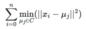
The K-means algorithm is designed to choose cluster centers that minimize the within-cluster sum-of-squares. This metric, referred to as inertia or distortion, is calculated by summing the squared distances from each sample point (xi) to its assigned cluster mean (μj):

As an example of calculating the inertia for the iris dataset, let’s assume we have preexisting knowledge that there should be exactly 3 clusters (one for setosa, one for versicolor, and one for virginica). We can fit a K-means model with 3 initial clusters as shown below:

>>> from sklearn import datasets
>>> from sklearn.cluster import KMeans
>>> iris = datasets.load_iris()
>>> kmeans = KMeans(n_clusters=3)
>>> kmeans.fit(iris.data)
KMeans(algorithm='auto', copy_x=True, init='k-means++',
       max_iter=300, n_clusters=3, n_init=10, n_jobs=None,
       precompute_distances='auto', random_state=None,
       tol=0.0001, verbose=0)
>>> kmeans.cluster_centers_
array([[5.9016129 , 2.7483871 , 4.39354839, 1.43387097],
       [5.006     , 3.428     , 1.462     , 0.246     ],
       [6.85      , 3.07368421, 5.74210526, 2.07105263]])

We can then plot the centroids learned from our model as well as the model prediction as a gut check to test how our model performed. Note that the K-means algorithm can be used with multi-dimensional data (as we have done here with 4 features from the iris dataset). However, it is a lot easier to illustrate how the algorithm works if we stick to 2D in our plot.  Thus, we only plot the results considering the first two features – sepal length and sepal width.

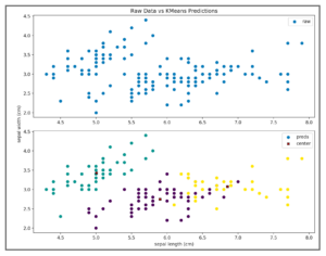
In order to calculate the inertia for our model, we need to square the distance from each sample point and its associated cluster center, and then sum all these values. That means, we’d need to calculate the distance from each green point above and the cluster center located at (5.006, 3.428) and then square those distances. We’d do the same for the purple points, calculating the distance from the cluster center located at (5.9016129, 2.7483871) and square. Finally, we’d continue with the yellow points using the cluster center located at (6.85, 3.07368421). We can use scipy.spatial.distance.cdist() to accomplish this task:

>>> import numpy as np|
>>> import scipy.spatial.distance
>>> distances = scipy.spatial.distance.cdist(
...     XA=iris.data,
...     XB=kmeans.cluster_centers_,
...     metric='euclidean'
... ) 

>>> distances
array([[3.41925061, 0.14135063, 5.0595416 ],
       [3.39857426, 0.44763825, 5.11494335],
       [3.56935666, 0.4171091 , 5.27935534],
       ...
       [1.17993324, 4.41184542, 0.65334214],
       [1.50889317, 4.59925864, 0.83572418],
       [0.83452741, 4.0782815 , 1.1805499 ]])
>>> distances_closest_centroid = distances.min(axis=1)
>>> distances_closest_centroid
array([0.14135063, 0.44763825, 0.4171091 , ... 
       0.65334214, 0.83572418, 0.83452741])
>>> manual_inertia = np.square(distances_closest_centroid).sum()
>>> manual_inertia
78.85144142614601

Luckily for us, sklearn stores this metric as a learned attribute via kmeans.intertia_

>>> kmeans.inertia_
78.85144142614601

>>> print(f"Manually calculated inertia: {manual_inertia}\n"
...       f"sklearn stored inertia     : {kmeans.inertia_}")
Manually calculated inertia: 78.85144142614601
sklearn stored inertia     : 78.85144142614601

Why Should We Care About Inertia?

When it comes to K-means clustering, a lower inertia is better. This intuitively makes sense because we defined this metric as the sum of squared distances from each point to its assigned centroid – the smaller the inertia the more tightly we have clustered our sample points to the discovered centroids. But, there is one slight problem.

If we were to choose a higher number of clusters, say 16, we’d see that our inertia decreases significantly to 18.03:

>>> kmeans = KMeans(n_clusters=16)
>>> kmeans.fit(iris.data)

KMeans(algorithm='auto', copy_x=True, init='k-means++', 
       max_iter=300, n_clusters=16, n_init=10, n_jobs=None,
       precompute_distances='auto', random_state=None,
       tol=0.0001, verbose=0)
>>> kmeans.inertia_
18.029802726513253

By increasing the number of clusters, we have artificially improved our model. We know that the true number of clusters for the iris dataset is 3 and thus have some intuition that we aren’t really getting better results here. We are merely improving the squared distance metric by adding more centroids. This becomes more evident if we were to choose a k that was almost equal to the number of data points in our dataset.

>>> kmeans = KMeans(n_clusters=len(iris.data)-1)
>>> kmeans.fit(iris.data)
KMeans(algorithm='auto', copy_x=True, init='k-means++', 
       max_iter=300, n_clusters=149, n_init=10, n_jobs=None,
       precompute_distances='auto', random_state=None,
       tol=0.0001, verbose=0)
>>> kmeans.inertia_
0.0

So, choosing the number of clusters just based on the smallest inertia isn’t the ideal way to find the optimal number of clusters. Choosing too many clusters will lead to artificially deflating the inertia metric and could lead to substantial overhead if the number of clusters becomes too large. We also don’t want to choose too few clusters and yield an inertia value that is so high that our model isn’t learning anything. We need to strike a balance between a low inertia value and the number of clusters we choose.

The Elbow Method

In order to strike this balance between inertia and the number of clusters chosen, we can use the elbow method. In this approach, we will define a range of cluster numbers to test and iteratively fit a model for each entry while storing the inertia for each iteration. We will then plot these inertia values and look for the “elbow” point of the resulting plot. Specifically, we are looking for the inflection point of maximal curvature and that will be our optimal k (the ideal number of clusters for our problem).

>>> inertias = []
>>> k_range = range(1, 16)
>>> for k in k_range:
...     kmeans = KMeans(n_clusters=k)
...     kmeans.fit(iris.data)
...     inertias.append(kmeans.inertia_)

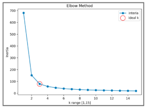
The resulting plot leads us to choose 3 as the ideal number of clusters for our K-means algorithm operating on the iris dataset.

Beyond K-means Clustering

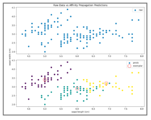
In some instances, you may have no intuition on the exact number of clusters in your dataset nor an acceptable range to test. Rather than fitting various K-means models, you may consider using the Affinity Propagation algorithm instead. This technique does not require you to provide a number of clusters and instead self-organizes to choose the number of clusters by sending “messages” (a responsibility metric and an availability metric) between pairs of samples. While this idea of message passing can seem a bit opaque, a good mental model is to think of the responsibility as the suitability for one sample to be the exemplar of another (can a data point be responsible for another data point) and the availability to be a measure of how appropriate it would be for a data point to choose another data point as its exemplar (is a datapoint available to be described by another data point).

Unlike K-means, the goal of Affinity Propagation is to choose actual sample data points that best describe and are most representative of the dataset. These chosen points are called “exemplars” and are similar to the centroids in the K-means clustering algorithm (except that in this case they are actual data points from the dataset). For more information, see the sci-kit learn documentation.

>>> from sklearn.cluster import AffinityPropagation
>>> ap = AffinityPropagation(preference=-20)
>>> ap.fit(iris.data)
AffinityPropagation(affinity='euclidean', convergence_iter=15, copy=True, damping=0.5, max_iter=200, preference=-20, verbose=False)
>>> ap.cluster_centers_
array([[5. , 3.4, 1.5, 0.2],
       [6. , 2.9, 4.5, 1.5],
       [6.9, 3.2, 5.7, 2.3]])

# Unlike K-means centroids, AP exemplars are actual data points
>>> ap.cluster_centers_indices_
array([  7,  78, 120])
>>> iris.data[ap.cluster_centers_indices_]
array([[5. , 3.4, 1.5, 0.2],
       [6. , 2.9, 4.5, 1.5],
       [6.9, 3.2, 5.7, 2.3]])

If you have no preexisting knowledge of the number of clusters in your dataset, trying Affinity Propagation clustering may be a good idea. You should consider using this algorithm if you want to guarantee that cluster centers are chosen from data points in the training dataset or if you have many clusters or uneven/unbalanced cluster groupings in the data. One caveat to Affinity Propagation is that it does not scale well. The algorithm has a time complexity of the order O(N²T), where N is the number of samples and T is the number of iterations until convergence. Further, the memory complexity is of the order O(N²).This makes Affinity Propagation most appropriate for small to medium sized datasets.

Conclusion

K-means clustering is a great general-purpose algorithm that scales well with large datasets. We’ve used the iris dataset to explore this popular clustering technique and demonstrated how to calculate the inertia for a given model. By using the elbow method, we explored how to choose the ideal k by striking a balance between a model’s inertia and the chosen number of clusters. We’ve also introduced Affinity Propagation clustering which can be used if we have no preexisting intuition on the number of clusters that exist in our dataset. Be careful, though, as this method is complex and doesn’t scale well. Your best bet might be to try K-means – and a little elbow grease method – to derive a suitable number of clusters.

About the Author

Logan Thomas holds a M.S. in mechanical engineering with a minor in statistics from the University of Florida and a B.S. in mathematics from Palm Beach Atlantic University. Logan has worked as a data scientist and machine learning engineer in both the digital media and protective engineering industries. His experience includes discovering relationships in large datasets, synthesizing data to influence decision making, and creating/deploying machine learning models.